Merge Sort
Algorithm
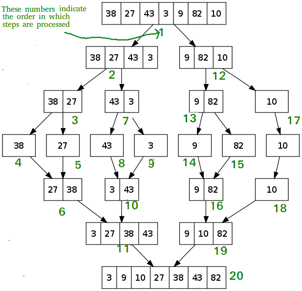
Like QuickSort, Merge Sort is a Divide and Conquer algorithm. It divides the input array into two halves, calls itself for the two halves, and then merges the two sorted halves. The merge() function is used for merging two halves. The merge(arr, l, m, r) is a key process that assumes that arr[l..m] and arr[m+1..r] are sorted and merges the two sorted sub-arrays into one. See the following C implementation for details.
Time Complexity :
Sorting arrays on different machines. Merge Sort is a recursive algorithm and time complexity can be expressed as following recurrence relation.
T(n) = 2T(n/2) + θ(n)
The above recurrence can be solved either using the Recurrence Tree method or the Master method. It falls in case II of Master Method and the solution of the recurrence is θ(nLogn). Time complexity of Merge Sort is θ(nLogn) in all 3 cases (worst, average and best) as merge sort always divides the array into two halves and takes linear time to merge two halves. Auxiliary Space: O(n) Algorithmic Paradigm: Divide and Conquer Sorting In Place: No in a typical implementation Stable: Yes
Time Complexity :
Best Time: O(NlogN)
Average Time: O(NlogN)
Worst Time: O(NlogN)
Bubble Sort
Algorithm
Bubble Sort is the simplest sorting algorithm that works by repeatedly swapping the adjacent elements if they are in wrong order.
This sorting algorithm is comparison-based algorithm in which each pair of adjacent elements is compared and the elements are swapped if they are not in order.
This algorithm is not suitable for large data sets as its average
and worst case complexity are of Ο(n2) where n is the number of items.
Example:
First Pass: ( 5 1 4 2 8 ) –> ( 1 5 4 2 8 ),
Here, algorithm compares the first two elements, and swaps since 5 > 1. ( 1 5 4 2 8 ) –> ( 1 4 5 2 8 ),
Swap since 5 > 4 ( 1 4 5 2 8 ) –> ( 1 4 2 5 8 ),
Swap since 5 > 2 ( 1 4 2 5 8 ) –> ( 1 4 2 5 8 ),
Now, since these elements are already in order (8 > 5),
algorithm does not swap them.
Pass: ( 1 4 2 5 8 ) –> ( 1 4 2 5 8 ) ( 1 4 2 5 8 ) –> ( 1 2 4 5 8 ),
Swap since 4 > 2 ( 1 2 4 5 8 ) –> ( 1 2 4 5 8 ) ( 1 2 4 5 8 ) –> ( 1 2 4 5 8 )
Now, the array is already sorted, but our algorithm does not know if it is completed.
The algorithm needs one whole pass without any swap to know it is sorted.
Third Pass: ( 1 2 4 5 8 ) –> ( 1 2 4 5 8 ) ( 1 2 4 5 8 ) –> ( 1 2 4 5 8 ) ( 1 2 4 5 8 ) –> ( 1 2 4 5 8 ) ( 1 2 4 5 8 ) –> ( 1 2 4 5 8 )
Time Complexity :
Best Time: O(N)
Average Time: O(N^2)
Worst Time: O(N^2)
Quick Sort
Algorithm :
QuickSort is a Divide and Conquer algorithm. It picks an element as pivot and partitions the given array around the picked pivot. There are many different versions of quickSort that pick pivot in different ways. Always pick first element as pivot. Always pick last element as pivot (implemented below) Pick a random element as pivot. Pick median as pivot. The key process in quickSort is partition(). Target of partitions is, given an array and an element x of array as pivot, put x at its correct position in sorted array and put all smaller elements (smaller than x) before x, and put all greater elements (greater than x) after x. All this should be done in linear time.
Partition Algorithm
There can be many ways to do partition, following pseudo code adopts the method given in CLRS book. The logic is simple, we start from the leftmost element and keep track of index of smaller (or equal to) elements as i. While traversing, if we find a smaller element, we swap current element with arr[i]. Otherwise we ignore current element.
                         low --> Starting index, high --> Ending index
                          quickSort(arr[], low, high)
                          { if (low < high)
                             { /* pi is partitioning index, arr[pi] is now at right place */
                                pi=p artition(arr, low, high);
                                 quickSort(arr, low, pi - 1); // Before
                                 pi quickSort(arr, pi + 1, high); // After pi
                                }
                            }
Time Complexity :
Best Time: O(NlogN)
Average Time: O(NlogN)
Worst Time: O(N^2)
Insertion Sort
Algorithm :
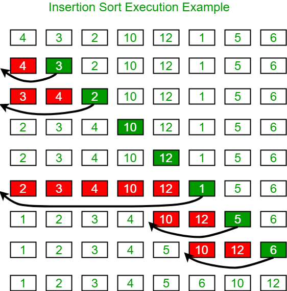
Insertion sort is a simple sorting algorithm that works similar to the way you sort playing cards in your hands. The array is virtually split into a sorted and an unsorted part. Values from the unsorted part are picked and placed at
the correct position in the sorted part. Algorithm To sort an array of size n in ascending order:
1: Iterate from arr[1] to arr[n] over the array.
2: Compare the current element (key) to its predecessor.
3: If the
key element is smaller than its predecessor, compare it to the elements before. Move the greater elements one position up to make space for the swapped element.
Time Complexity :
Best Time: O(N)
Average Time: O(N^2)
Worst Time: O(N^2)
Quick Sort
Algorithm :
QuickSort is a Divide and Conquer algorithm. It picks an element as pivot and partitions the given array around the picked pivot. There are many different versions of quickSort that pick pivot in different ways. Always pick first element as pivot. Always pick last element as pivot (implemented below) Pick a random element as pivot. Pick median as pivot. The key process in quickSort is partition(). Target of partitions is, given an array and an element x of array as pivot, put x at its correct position in sorted array and put all smaller elements (smaller than x) before x, and put all greater elements (greater than x) after x. All this should be done in linear time.
Partition Algorithm
There can be many ways to do partition, following pseudo code adopts the method given in CLRS book. The logic is simple, we start from the leftmost element and keep track of index of smaller (or equal to) elements as i. While traversing, if we find a smaller element, we swap current element with arr[i]. Otherwise we ignore current element.
                         low --> Starting index, high --> Ending index
                          quickSort(arr[], low, high)
                          { if (low < high)
                             { /* pi is partitioning index, arr[pi] is now at right place */
                                pi=p artition(arr, low, high);
                                 quickSort(arr, low, pi - 1); // Before
                                 pi quickSort(arr, pi + 1, high); // After pi
                                }
                            }
Time Complexity :
Best Time: O(NlogN)
Average Time: O(NlogN)
Worst Time: O(N^2)
Heap Sort
Algorithm :
Heap sort is a comparison-based sorting technique based on Binary Heap data structure. It is similar to selection sort where we first find the minimum element and place the minimum element at the beginning.
We repeat the same
process for the remaining elements. What is Binary Heap? Let us first define a Complete Binary Tree. A complete binary tree is a binary tree in which every level, except possibly the last, is completely filled, and all nodes are
as far left as possible (Source Wikipedia) A Binary Heap is a Complete Binary Tree where items are stored in a special order such that the value in a parent node is greater(or smaller) than the values in its two children nodes.
The former is called max heap and the latter is called min-heap. The heap can be represented by a binary tree or array. Why array based representation for Binary Heap? Since a Binary Heap is a Complete Binary Tree, it can be easily
represented as an array and the array-based representation is space-efficient. If the parent node is stored at index I, the left child can be calculated by 2 * I + 1 and the right child by 2 * I + 2 (assuming the indexing starts
at 0).
Heap Sort Algorithm for sorting in increasing order: 1. Build a max heap from the input data. 2. At this point, the largest item is stored at the root of the heap. Replace it with the last item of the heap followed by
reducing the size of heap by 1. Finally, heapify the root of the tree. 3. Repeat step 2 while the size of the heap is greater than 1. How to build the heap? Heapify procedure can be applied to a node only if its children nodes
are heapified. So the heapification must be performed in the bottom-up order.
            Input data: 4, 10, 3, 5, 1
                    4(0)                                                     |   public void sort(int arr[])
                   /   \                                                     |    {
                10(1)   3(2)                                                 |          int n = arr.length;
               /   \                                                         |           // Build heap (rearrange array)
               5(3)    1(4)                                                            for (int i = n / 2 - 1; i >= 0; i--)
                                                                             |               heapify(arr, n, i);
                                                                             |         // One by one extract an element from heap
                                                                                       for (int i = n - 1; i > 0; i--) {
           The numbers in bracket represent the indices in the array         |           // Move current root to end
                                                                             |                 int temp = arr[0];
           representation of data.                                           |                 arr[0] = arr[i];
                                                                             |                 arr[i] = temp;
           Applying heapify procedure to index 1:                            |                 // call max heapify on the reduced heap
                    4(0)                                                     |                  heapify(arr, i, 0);
                   /   \                                                     |              }
               10(1)    3(2)                                                 |      }
               /   \                                                         |
           5(3)    1(4)                                                      |
                                                                             |
           Applying heapify procedure to index 0:                            |
                   10(0)                                                     |
                   /  \                                                      |
                5(1)  3(2)                                                   |
               /   \                                                         |
            4(3)    1(4)                                                     |
           The heapify procedure calls itself recursively to build heap      |
            in top down manner.
Time Complexity :
Best Time: O(NlogN)
Average Time: O(NlogN)
Worst Time: O(NlogN)
Selection Sort
Algorithm :
The selection sort algorithm sorts an array by repeatedly finding the minimum element (considering ascending order) from unsorted part and putting it at the beginning. The algorithm maintains two subarrays in a given array.
1) The subarray which is already sorted.
2) Remaining subarray which is unsorted.
In every iteration of selection sort, the minimum element (considering ascending order) from the unsorted subarray is picked and moved to the sorted subarray.
            arr[] = 64 25 12 22 11

            // Find the minimum element in arr[0...4]
            // and place it at beginning
            11 25 12 22 64

            // Find the minimum element in arr[1...4]
            // and place it at beginning of arr[1...4]
            11 12 25 22 64

            // Find the minimum element in arr[2...4]
            // and place it at beginning of arr[2...4]
            11 12 22 25 64

            // Find the minimum element in arr[3...4]
            // and place it at beginning of arr[3...4]
            11 12 22 25 64